Advanced Control: SOPDT Auto Tuning

Peter Nachtwey · Sep 15, 2018

Attached is a zip file that contains a python script that calculates the PID gains for SOPDT systems. You must install python3, numpy, scipy and matplotlib or Anaconda to run the script. The input file must be a text type file like a comma, tab or space separated variable file that has 3 columns. Time, control output in percent and the process variable. You need to edit the path to the data and make sure that the delimiter is set right. The script will take about a minute to run.

I have included a file called hotrod.txt. This file was originally generated by Ron Beaufort from his 'hotrod' tuning class. This files is about 10 years old.

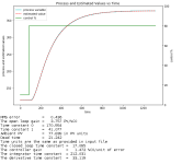
The output is a some mathematical data about how good the fit is. There is also a plot that shows how well the model can estimate the actual response using the same input. The estimated response and actual response ( PV ) should be close to identical. The final output shows the plant open loop gain, two time constants, an offset ( ambient temperature in this case ) and a dead time.

A closed loop time constant needs to be calculated to determine how strongly the PID parameters will react to errors. The PID parameters are then calculated. Make the closed loop time constant smaller for a stronger response and longer for a weaker response to errors.

The PID gains are calculated assuming the ISA model of dependent gains.

The PID parameters may not be directly useable for all PLCs or closed loop controller. First, most PLCs use time constants in minutes. Because the time base in the hotrod.txt is in seconds, the time constants need to be converted to minutes. If your input file uses minutes then no adjustments are necessary. The calculated controller gain has units of percent control output per unit of error which is degrees fahrenheit in this case. Some controllers have controllers where the gain is counts of output per counts of error. This will require scaling or unit analysis to covert my calculated gains to PLC conts out/counts in gains.

rwatson · Sep 18, 2018

I'm curious about how you came up with the closed loop time constant and parameters. Are these just from a rule of thumb? They don't look like values that would be generated from pole placement like you normally use.

Peter Nachtwey · Sep 18, 2018

I used the Internal Model Control, IMC, method that the controlguru uses. Actually IMC attempts to place one real pole at -1/tc and cancel out the other two poles with zeros so the response looks like there is just one pole.

I dug this up. It is from 2007
http://deltamotion.com/peter/Mathcad/SOPDT/Mathcad - SOPDT_HOTROD.pdf
It is the derivation of the IMC SOPDT gains.

The formula for calculating the closed loop poles is aggressive but since the model is fits the actual data very well the tc can be more aggressive. I wrote a program to do the same thing in Scilab but I have decided to use python since it is a cleaner and more flexible language. If you think the closed loop time constant is too aggressive you can make it bigger to slow down the response.

There is another recent thread where the OP has long dead times. In these cases a Smith Predictor should be used but before the Smith Predictor can be used one must compute a decent model. That is where this system identification program comes in handy.
http://deltamotion.com/peter/Mathcad/SOPDT/Mathcad - SOPDT SP.pdf

Edit, one more thing.
I run the minimize function twice. This keep the minimizer from getting stuck in a local minimum.

I am trying to do more of my work using Python now because it is free, easy to use and text based so I can copy code into a forum

Code:

def difeq(y, t, k, t0, t1, c, dt ):
    """ generate estimated SOPDT solution
        y[0] = process value
        y[1] = rate of change of the process value"""
    t = max(t-dt,0)
    _u = control_interp(t)              # offset CO for dead time
    _dy2dt = (-(t0+t1)*y[1]-y[0]+k*_u+c)/(t0*t1)    # SOPDT dif Eq
    return np.array([y[1], _dy2dt])

BTW, cost function that is minimized is
_sse = np.sum((aPV-_aEV[:,0])**2)
This calculates the sum of squared errors between the estimate value and the process variable. The smaller this number is the better the fit.

If you enable the print statement below this equation you can see the sum of squared error converge to a minimum. If you use the plot_data function to print all the different tries you can see how the estimate response converges on the actual response.
However, this is very slow but still interesting.

Advanced Control: SOPDT Auto Tuning

Peter Nachtwey

Member

Attachments

rwatson

Member

Peter Nachtwey

Member

Similar Topics