How to smooth out a very inconsistent reading

beauedgar89 · Aug 4, 2022

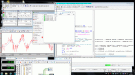
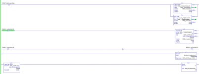
I am using an analog laser level detector to detect the rubber level in a 2 cylinder mill. The rubber is introduced on one side in softball sized balls that fall onto the cylinders and get worked into the gap. The laser I am using is very accurate but due to the randomness of how the balls fall and stack on the cylinders, it is difficult to get a consistent reading. The laser has to be mounted above the mill to be out of the way and shoots directly down to the rubber. I have attached a screen shout of my logic I am attempting to use to smooth out the readings but I wanted to know if someone knows a way to get it even better, or if I should add more logic to the existing rungs.

Lare · Aug 4, 2022

You can try Mickey's filter after averaging.

http://www.plctalk.net/qanda/showthread.php?t=108849

OkiePC · Aug 4, 2022

I am sure there are more advanced ways to do what you want, but in my simple world I have good success with a first order filter I got from Mickey on this site:
FIRST ORDER FILTER TO SMOOTH ANALOG JITER:
FV=FV+C(NV-FV)
Where:
FV= Filtered value
C= constant (range 0-1) The smaller the number the more dampening. A value of 1.000 indicates no filtering.
NV= New Value

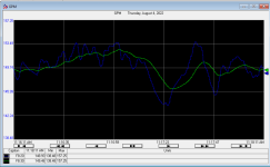
Here's a trend for a system I am working on today where the gpm signal is wandering around quite a bit and I don't want my chemical pacing controls based on that wandering signal to follow suit, so I have a filter constant of 0.05 applied and the blue line is prior to filtering, the green line is filtered. I update the result every ~20ms on a oneshot from a bit in the Micrologix free running clock.

You should trend your signal raw and filtered or averaged to get a visual of the impact it is having (or going to have) on the process.

Peter Nachtwey · Aug 4, 2022

Nice trend OkiePC!

tvey · Aug 4, 2022

1D Kalman Filter

Here's a sample implementation of a 1D Kalman filter.

It's in SCL but the (much simplified) algorithm would be reasonably straightforward to implement in ladder. I'm attaching a short .gif of the filter in operation on a simulator.

A good starting point for some initial tuning parameters:

q = 0.125, r = 32, p = 1023

where:

q = process noise covariance
r = measurement noise covariance
p = estimation error covariance

Adjust as necessary to suit your process.

-Trevor

Peter Nachtwey · Aug 4, 2022

@tvey, I can't even get these guys to calculate the C value in OkiePC's example correctly. I doubt they will go through the effort.
Also, I have been on many engineering forums where Kalman filters were discussed. Engineers do not know the values to use for process and measurement noise so they fudge it which is not that much different from the people on this forum fudging the value of C.
Your Kalman filter is still basically a simple low pass filter.In your example the Kalman gain will soon reach a steady state value dependent of the initial values of q and r so why not just enter the k value directly? I don't see where your k gain changes as a function of the measurement noise.

I wanted something like this for our motion controllers. It would be handy to have a filter with minimal phase lag for filtering encoder counts. Knowing that people will just fudge parameters until they get the desired results, I implemented a alpha-beta-gamma and alpha-beta-gamma-delta filter. The basic form is alpha-beta filter.
https://en.wikipedia.org/wiki/Alpha_beta_filter
This family of filters is basically a steady state Kalman filter that makes no pretense of knowing the measurement or process noise. The customer just picks a bandwidth until he gets the desired response. The huge advantage of the alpha-beta class of filters is that they don't suffer from phase lag as much as normal low pass filters because there is a prediction phase where x is updated(estimated) and then corrected using the k gains.
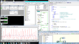
This is a 3rd order alpha-beta-gamma filter. I simulate noise and feed back resolution quantizing.
ABG (deltamotion.com)
This is basically the same thing on a 4th order alpha-beta-gamma-delta filter
ABGD (deltamotion.com)
I used the same noise generated in the 4th order example as used in the 3rd order example. Notice that the 4th order filter is more accurate.
The key is that having higher order filters allow for better prediction and therefore less phase lag. You can see there is little

BTW, the examples were don't because we were controlling a crane like device that only had feedback every 10 ms from a MRU ( motion reference unit ) where as we needed feedback every 1 ms so we had to estimate the state every millisecond better the 10 millisecond readings.

We haven't found any MRUs that can do a better job of filtering that us so far.

alpha-beta-gamma filter in action. The feedback is coarse, only 2000 counts per revolution and the update rate is every 250 microseconds. The ability to calculate speed is hindered by the low resolution but I can even estimate an acceleration. Using the encoder counts directly is pointless. I show the difference between the alpha-beta-gamma filter and a four pole Butterworth filter. This example is extreme because rarely do motors move in such a random way.

https://deltamotion.com/peter/Videos/AlphaBetaGamma.mp4

I have posted these links before and still, no one has made an AOI or a Siemens FB from the code after all these years.

JesperMP · Aug 8, 2022

Peter Nachtwey said:
I have posted these links before and still, no one has made an AOI or a Siemens FB from the code after all these years.

I have made an FB for Siemens for the Alpha-Beta filter. It is SCL i.e. Structured Text, so it should be easily imported into Rockwell.

Code:

FUNCTION_BLOCK FB_ALPHA_BETA_FILTER
// based on https://en.wikipedia.org/wiki/Alpha_beta_filter

VAR_INPUT
    xm: REAL ; // raw input value
    deltat : REAL ; // update time [seconds]
    a : REAL := 0.85 ; // alpha constant
    b : REAL := 0.005 ; // beta constant
END_VAR

VAR
    xk : REAL := 0.0 ; // estimated position part
    xk_1 : REAL := 0.0 ; // estimated position part of previous iteration
    vk : REAL := 0.0 ; // estimated velocity part
    vk_1 : REAL := 0.0 ; // estimated velocity part of previous iteration
    rk : REAL := 0.0 ; // prediction error
END_VAR 

VAR_OUTPUT 
    filter_out : REAL ; // filtered output
    status : INT ; // 0=error, 1=ok, 2=ok but noise is not suppressed
END_VAR 

IF // check input parameters
    deltat > 0.0 AND 
    a > 0.0 AND 
    a < 1.0 AND 
    b > 0.0 AND 
    b < 2.0 AND 
    4 - 2*a - b > 0 THEN 

   // if input parameters are OK, then perform the calculation
    xk := xk_1 + (vk_1 * deltat);
    vk := vk_1 ;
    rk := xm - xk;
    xk := xk + (a * rk);
    vk := vk + (b * rk / deltat);
    xk_1 := xk;
    vk_1 := vk;
    
    IF b < 1.0 THEN
        status := 1; // parameters OK
    ELSE
        status := 2; // parameters OK but noise is not suppressed        
    END_IF ;

    filter_out := xk_1 ;

ELSE // input parameter check failed
    filter_out := 0.0 ;
    status := 0 ; // parameter error
END_IF; 

END_FUNCTION_BLOCK

I would give it a go at the Alpha-Beta-Delta filter, but I cannot interpret the Matchcad code you posted. Any code sample or pseudo-code in C or ST or similar ?

Peter Nachtwey · Aug 9, 2022

@JesperMP. Excellent! However I think there needs to be some corrections.
I am not home now. I will try to supply the code when I am able. I need to find code easier to understand.

Peter Nachtwey · Aug 9, 2022

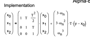
I did some searching and I found on my laptop an old pdf that explains the alpha-beta-gamma filter a little. Page 8/9 shows the implementation.
The first equation describes the filter in matrix and vector form
There is a x vector where x0 is the position, x1 is the velocity and x2 is the acceleration. However, x could be about anything and its first and second derivatives.
The 3x3 matrix is normally labeled as A or the transition matrix. It predicts the next values for the x vector. If you multiply it out you will see the top line yields

Code:

 x0(n+1)=x0(n)+x1(n)*T+(1/2)*x2(n)*T^2

T is the same period.

The next vector is the K gains. The omegas select the bandwidth on how fast the errors in perdiction are corrected. Omega is what the user adjusts to get the desired results. Notice the weights of 3 3 and 1. Don't change this for now. The ratio of the K gains for the errors in position, velocity and acceleration are key. The whole vector is multiplied by T which is the sample time. Finally the K gains are multiplied by the error between the estimated position x0 and the measured position y. This part of the equation corrects for errors in the predicted values. In this example my model is just predicting that the position velocity and acceleration will do what they did before which is works petty well for smoothing the encoder counts on a feed chain where there is noise as the links go over sprockets but overall the chain is moving at a pretty consistent rate.

The 3x3 matrix is really the key since it predicts and reduces the phase lag significantly.

My pdf file was too big so I had to take a snap shot of just the formula.

http://www.plctalk.net/qanda/attachment.php?attachmentid=62757&stc=1&d=1660055970

JesperMP · Aug 9, 2022

@Peter Nachtwey.
I tried to search by myself, but I became unsure if I was on the right track. Some papers I found seemed to discuss kalman filter and alpha-beta-gamma filter in the same context as if they were the same thing.
I think I can work out what you have written.

A few questions:
Where are the "α", "β" and "γ" factors in the formula ?
And you write "The omegas select the bandwidth on how fast the errors in perdiction are corrected. Omega is what the user adjusts to get the desired results."
So there are "α", "β", "γ" and "ω" factors that are all user-set is that correct ?
What does the "n" denote in the matrix formula at "ω_n" ?
Also, generally speaking, is an alpha-beta-gamma filter a simplified kalman filter ? Or how are they related ?

JesperMP · Aug 9, 2022

Previously you wrote:
"However I think there needs to be some corrections."
Can you elaborate on that ?

drbitboy · Aug 9, 2022

Here is a MatLab version of the alpha-beta-gamma filter. It appears to be consistent with what @Peter Nachwey posted.

drbitboy · Aug 9, 2022

The penny is finally starting to drop:

alpha, beta, and gamma, are weights apportioning ongoing and filtered corrections to estimates of position, velocity, and acceleration, respectively, to correct for ongoing error (from both estimate and measurement) in the position estimate relative to the position measurement.
the alpha-beta filter is an alpha-beta-gamma filter with gamma=0.
an alpha filter is an alpha-beta filter with beta=0.
an alpha filter is an exponential filter: estimate(k) = f * measurement(k) + (1-f) * estimate(k-1)

That almost makes more sense if read from bottom to top.

Peter Nachtwey · Aug 13, 2022

JesperMP said:
Previously you wrote:
"However I think there needs to be some corrections."
Can you elaborate on that ?

It isn't clear how you calculated alpha and beta also I don't agree with your checks. The little n shouldn't be there. It should just be omega which represents the frequency of the filter. Normally the beta or K1 gain will be multiplied by the error in velocity. It is greater than the K0 or alpha gain.

Code:

[K0,K1][sup]T[/sup] = [ sqrt(2)*omega, omega^2][sup]T[/sup]

omega is the frequency of the filter or how fast it will respond to errors. omega is the user adjustable parameter that is changed to get the desired result. You can see that omega^2 will be higher than sqrt(2)*omega most of the time.

drbitboy is right about now the name relates to the number and order of the gains.

So who is going to make a FB and AOI? I think a 3rd order alpha-beta-gamma filter is a good place to start.

I don't have a need for the alpha-beta filter but I do use the alpha-beta-gamma filter so I can gear to the master's position, velocity AND acceleration. Most people just gear to the position and wonder why they have phase lag between the master and slaves.

I've been camping in the sticks, no water, phone, electricity, air conditioning ( it was hot ), TV, internet etc. Sometimes I could get radio. I can always get weather radio. I do have a satellite phone so I can let people know where I am. The weather radio and satellite phone are a must have.

Peter Nachtwey · Aug 15, 2022

I attached a simpler alpha-beta example

This pdf was made in 2016 for this forum. I assumed the samples were taken every 10 ms and that the resolution is of the encoder is 0.01mm so the best velocity resolution is 1 meter per second which is horrible. This means the speed would appear to change in increments of 1 m/s.

To make it a challenge I wanted the alpha-beta filter to follow a 1 Hz sine wave with an amplitude of 10 mm. The peak speed is only 62.8 mm/s so if no filter is used then one would see the speed change from 0 to 1 m/s back to 0 then to -1 m/s. This is not usable. One could average 10 readings but a whole sine wave requires only 100 reading at 10 ms per reading so averaging 10 numbers would add a significant delay. Even so it resolution would now be 0.1 m/s instead of 1 m/s. This still isn't acceptable. Image what the result would be.

The first part of the pdf show the derivation. Ignore that if you want. On page 2/16 I calculated the optimum filter frequency, omega, to be 70.7 Hz. Notice the filter gain calculations for K0 and K1. The filter response will be like a two pole Butterworth filter with the ability to predict so there is little phase lag.

On page 3/16 the predicted positions are calculated and the error between the predicted and the actual sine wave position is less than 0.1 mm.

On page 4/16 the correction is added to the predicted position to get the final estimated position.

On page 5/16 a show how the estimated position tracks the target sine wave almost perfectly. The error between the estimated position is less than 0.01mm. Most of the time the error is much less. Remember the position feed back resolution from the encoder is 0.01mm. A slight improvement.

On page 6/16 the estimated velocity is calculated.

One page 7/16 I show the estimated vs target velocity. You can see there is a little phase lag but that is mostly due to the 10 millisecond sample time. The magic is that the error between the estimated velocity and the target velocity is just a little over 5 mm/s as opposed to the unfilter velocity resolution of 1 m/s. That is an improvement of almost 200 times and with little phase delay.

On page 9/16 I made a Bode plot of the filter's frequeny response. The Bode plot looks almost perfect. The spikes up and down are just round of error
because the errors have units of 10^-15. Again, in reality there is some phase delay due the sample time.

On page 10/16 on I show how to implement the alpha-beta filter using polynomials. The response is about the same. The difference is in how the filters are initialized. After a few iterations they are the same. The pdf shouldn't say alpha-beta-gamma. I need to change that.

I know I have posted this before but all information is lost after it falls off the front page.

How to smooth out a very inconsistent reading

beauedgar89

Member

Lare

Member

OkiePC

Lifetime Supporting Member

Peter Nachtwey

Member

tvey

Lifetime Supporting Member

Attachments

Peter Nachtwey

Member

JesperMP

Lifetime Supporting Member + Moderator

Peter Nachtwey

Member

Peter Nachtwey

Member

JesperMP

Lifetime Supporting Member + Moderator

JesperMP

Lifetime Supporting Member + Moderator

drbitboy

Lifetime Supporting Member

drbitboy

Lifetime Supporting Member

Peter Nachtwey

Member

Peter Nachtwey

Member

Similar Topics