Factory Talk View ME Mechanical simulation

[BMX1253]

Factory Talk View ME V.11
Studio 5000 V31
PlantPAx 4.0

I have a small customer designed system that I am trying to set up an offline simulation for.

System overview:
4 Exhaust fans, with a Pressure differential transmitter

PIDe PV = Pressure Differential Transmitter
PIDe CV = Output in Hz to each fan

I am trying to simulate a value for the Pressure differential transmitter to utilize. This would be based on a calculation I am writing into a macro that is updated every .5 second.

I got the macro updating and everything else, just struggling with the formula or how to make one for the PDT signal simulation.

I have 2 points that I want to be correct:
When 4 fans are running at 50Hz, the system will pull 3" of vacuum
When 3 fans are running at 60Hz, the system will pull 3" of vacuum

The calculated slope is Y = -10X + (-90) ; Y=MX+B

I don't know what kind of formula to use. Looking for any suggestions.

I've tried to use the variables
X = Number of enabled fans
Y = Hz output of PID loop
Z = Unknown constant or another equation?


Thanks.

 

[drbitboy]

A computer model

how is the air* coming into the space on which the vacuum is being pulled? Is it a process (e.g. heat exchanger, or burner flue), leakage, or a valve? If it's a process or a valve, does it ever change (i.e. control valve, run burner at a different rate)?



* I assume it's air



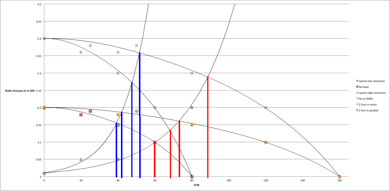
The actual system reaches an equilibrium when the flow rate of air coming into the system (call that flow leakage, or fIn) equals the rate of air being pulled out by the fans (fOut).


Assuming turbulent flow, the pressure differential (ΔP) is roughly proportional to the square of fIn, IIRC, ΔP = Cf**-2 fIn**2 (cf. [system resistance] curves below). Cf is the system flow coefficient (Cv) divided by the the square root specific gravity (sqrt(SG))for fIn. SG will change with pressure but we will ignore that for this model.

At the fans, the driven flow, fOut, decreases with increasing ΔP according to a fan curve e.g.

The fan speed (Hz, which may be one of the control inputs) moves that curve in and out wrt the origin (cf. [fan base] vs. [fan at 200%] curves above). The number of fans scales the flow along the abscissa without changing its extent along the ordinate (cf. [fan base] vs. [2 fans in parallel] curves above). Ignore the fans in series curve.


Those fan curves look like an inverse square root curve; that is not even close to exact but probably good enough for a simulation**. So ΔP = sqrt((fMax - fOut) / K); K is a fan curve coefficient roughly proportional to the fan speed; fMax is directly proportional both to the number of fans and to the fan speed (to first order).



At equilibrium, the ΔP and flow for both models will be the same, i.e.

• Cf**-2 fIn**2 = ΔP = sqrt((fMax' - fOut) / K)
  • equilibrium
• fIn = fOut = f'
  • equilibrium
• K Cf**-4 f'**4 = (fMax' - f')
• fMax' = f' + K Cf**-4 f'**4

That is the basic form of the equation we need to solve for f', and then drop f' back into the ΔP equation. We'll get to the prime in f' and fMax' in a bit.



More first-order modeling:

• FC = number of fans running
• FS = fan speed, Hz
• fMax' = A FC * FS
  • max flow at zero ΔP is proportion to FC and FS
• K = B / FS**2
  • max ΔP at zero flow is proportional to FS

So we need to solve for A and B, also f' at ΔP=3", but we only have two datapoints (3" ΔP with 4 fans at 50Hz, and with 3 fans at 60Hz). However, we don't need the actual values of fMax' and f', so if we make the following substitutions

• fMax = fMax' / A
• f = f' / A

then we can say

• fMax = FC FS

which basically re-scales the abscissa of the plot, replaces fMax' and f' with fMax and f, respectively, and rolls some power of the constant A into A and Cf, such that A becomes 1, and Cf is TBD, leaving us with only B and f to solve for from two data points in this equation:

• ΔP = sqrt((fMax - f) / K)

substituting ...

• ΔP = sqrt((FC FS - f) / (B / FS**2))
• ΔP = sqrt((FC FS**3 - f FS**2) / B)
• B ΔP**2 = FC FS**3 - f FS**2

Using the two known cases:

• B 3**2 = B 9 = 3 60**3 - f 60**2 = 648000 - 3600 f
• B 3**2 = B 9 = 4 50**3 - f 50**2 = 500000 - 2500 f

Subtracting previous equation from second-previous, solve for f and B:

• 0 = 148000 - 1100 f
• f = 134.545
• B = (648000 - 3600 134.545) / 9 = 18181.8
• B = (500000 - 2500 134.545) / 9 = 18181.8 (double check)

Solve for Cf**-4

• Cf**-2 f**2 = ΔP
• Cf**-2 = ΔP f**-2 = 3 134.545**-2 = 1.66e-4
• Cf**-4 = 2.746e-8

Now we move back to the model equation i.e.

• fMax = f + Cf**-4 K f**4
• fMax = f + Cf**-4 B FS**-2 f**4
• fMax = f + 4.99e-4 FS**-2 f**4
• FC FS = f + 4.99e-4 FS**-2 f**4

From the general form of that equations, fMax = f + m f**4, with fMax, f, and m all non-negative, f will always be between 0 and fMax, and dfMax/df is always positive



So one approach to a solution would be a binary search between 0 and fMax:

• Set fMax = FC FS
• set fHi = fMax
• Set fLo = 0
• Loop:
  • Set fEst = (fHi - fLo) / 2
  • calculate fMaxEst = fEst + 4.99e-4 FS fEst**4
  • if fMaxEst > fMax, set fHi = fEst
  • else set fLo = fEst
  • Exit loop when (fHi-fLo) is small (TBD)
    • 10 passes gets fEst to within (0.1% fMax) of f

Another approach would be Newton-Raphson, starting from fEst = fMax (= FC FS):

• fMaxEst = fEst + 4.99e-4 FS fEst**4
• dfMaxEst/df = 1 + 15.97 FS fEst**3
• ΔfMaxEst = (fMax - fMaxest) / (dfMaxEst/df)
• fEst = fExt + ΔfMaxEst
• Loop until ΔfMaxEst is small

Either way, once you have fEst, calculate the differential pressure

• ΔP = 1.66e-4 fEst**2

** Every computer program is a model of something in the real world; the only real choice is the level of fidelity; everything else flows from that.

 

[drbitboy]

The algorithms to solve for f proposed in the previous post are probably way more than what is needed; coding a spreadsheet with those loop steps, with cell row being FC and cell column being FS, and running it a few dozen times should provide a 2D map of the solution that could be fit with four polynomials, one for each value of FC, so you don't bother with loops in the PLC.

 

[drbitboy]

Dynamic model

d'Oh! That's all interesting but it assumes the process is always in equilibrium. I realized that a simpler solution is to model the dynamics.
​

Pressure is the accumulation of flow, if more air is flowing out than is leaking in, the pressure will decrease, which means the vacuum will decrease i.e.

• PV' = nRT
  • Ideal Gas Law
• P = nRT/V'
• dP/dt = RT/V' dn/dt
• ΔP = Patm - P
  • Vacuum measurement
• dΔP/dt = (fOut - fIn) / V
  • Assume dn/dt is proportional to -(fOut - fIn)

where the constant V represents the volume of the space being evacuated scaled by some proportionality constant (maybe RT from the ideal gas law?). Rearranging into a numerical integration that is performed once per AOI execution:

• fOut = fMax - (K ΔPold**2)
• fIn = Cf sqrt(ΔPold)
• Δ(ΔP) = Δt (fOut - fIn) / V
  • Δt is the time since the last calculation, 0.5s according to the OP
  • e.g. (S:35 * 1e-4) on a MicroLogix 1100
• ΔPnew = ΔPold + Δ(ΔP)

Over time that will converge on the equilibrium solution from post #2; it will be unstable if the constant V is set too small; it could be made stable with an Implicit Euler scheme, but that would probably not be worth the effort if V is large enough.


Caveat: this models the evacuated space dynamics, not the fan dynamics, nor the pressure sensor dynamics.

 

[BMX1253]

Truly impressed

Wow, Answers like that are why I love this forum.

For a better understanding of the system, they are 4 fans that are pulling about 680 CFM each to an operations room with tools that require exhaust for fumes. There are a fair amount of tools, and will go on and off individually. But the system is large enough that 1 or 2 tools changing cycles won't really effect our test points.


In order to get a number to change I was just taking the Number of Fans * the Hz they are running at, and multiplying by a constant of .01666.

This meant that I had to change the values the "system" was running at for 4 fans to 45Hz, but it is just to prove the system will operate as designed and will be tuned as the system is truly operating.

What I was trying to do was get a better "constant" or a simple equation that I can replace the .01666 with to get closer to the desired curve. The mechanical design company has already done the flow calculations required for approval. We're just a controls integrator and I was trying to make the customer happy and make numbers change on a screen before the system is built.

I think I am going to try and research how to write a VBA script in the HMI for simulation purposes, because what you explained would be handy for a few other systems that we do fairly routinely. I will just have to do some research into those calculations to get a better understanding on how to do it.

 

[drbitboy]

Try this:

(Fan_Count * Fan_Hz - 3 * Fan_Count**2) * 0.019672

It yields

• 3.01 for 3 @ 60Hz
• 2.99 for 4 @ 50Hz

Close enough?



The dynamic simulation, implemented for MicroLogix 1100, is here.

 

[BMX1253]

That's perfect for what I am trying to accomplish!

Question, how did you figure out the multiplier that works for both and the static (-3)?

I did snag the 1100 code, I will be checking at our office, I think I have one or 2 Micros laying around that I can stand up for VFD feedback and flow control FB for testing. (currently doing the VFD as macros as well) HAHA.

There are a ton of variables that you're calculating. I wish I knew more about how to calculate that stuff.

I greatly appreciate the help you've provided.

Thanks!

 

[drbitboy]

Question, how did you figure out the multiplier that works for both and the static (-3)?

Trial and error.


if X is fan count (3 or 4), and Y is fan speed (50 or 60), then the two X*Y products are not too far away from each other

• 4 * 50 = 200
• 3 * 60 = 180

So they are off by 20.


So, I empirically considered adjusting the total by a factor of N*X**2, where N is 1, 2, 3, etc, so calculating N*X**2 for X=3 and X=4:

• N=1: 1*3*3=9; 1*4*4=16
• N=2: 18; 32
• N=3: 27; 48

Those last two, 27 and 48, differ by 19, which is close to the 20 noted above, suggesting X*Y - 3*X**2 should be pretty close:

• 4*50 - 3*4**2 = 200 - 48 = 152
• 3*60 - 3*3**2 = 180 - 27 = 153

Cinderella! All that is left is to get the factor that gets us to 3" H2O, using the mean of those two X*Y-3*X**2 values:

• 152.5 * Q = 3
• Q = 3/152.5 = 0.019672

There is of course an analytical way (see below) to get a slightly smaller value for N that will give the same result for (X*Y - N*X**2) for {X=3,Y=60} and {X=4,Y=50}, but this was close enough.

• 4*50 + N*4**2 = 3*60 + N*3**2
• 200 + N*16 = 180 + N*9
• N*7 = -20
• N = -20/7 = -2.84514285714...

So X*Y - 20*X**2/7 is exact:

• 3*60 - 20*3**2/7 = 154.2857
• 4*50 - 20*4**2/7 = 154.2857

and then

• 154.2857 * Q = 3
• Q = 3/154.2857 = 0.01944444

 

[drbitboy]

There are a ton of variables that you're calculating. I wish I knew more about how to calculate that stuff.

It's all either multiplying by one or adding zero.

 

[drbitboy]

N.B. the model with those coefficients, (XY - 2.857X**2)*0.019,
is not at all realistic, as entering larger X (fan count) values will eventually produce lower ΔP results. For example, try {X:14,Y:40} or {X:21,Y:60} - the result is 0 for both.


This is true for any (XY - kX**2) model.

 

[drbitboy]

It's all either multiplying by one or adding zero.

Or as my dad used to say, there is only one mathematical operation: counting.